Concentration inference from amplitude signals

import matplotlib.pyplot as plt
import numpy as np

import pyudv.attenuation.direct_models as DM
from pyudv.attenuation.inversion import explicit_inversion
from pyudv.attenuation.sediment_acoustic_models import quartz_sand as quartz


def C_to_phi(C, rho=2.65e3):
    return C / rho


def phi_to_C(phi, rho=2.65e3):
    return phi * rho


fig_width_small = 11.25

Define the parameters for the direct model

d = 100e-6  # grain mean diameter [m]
rho = 2.65  # grain density [g/cm3]
rho = rho * 1e-3 / 1e-6  # grain density [kg/m3]

F = 2e6  # frequency [Hz]
T = 20  # Temperature [Celsius degrees]
a_w = DM.alpha_w(F, T)  # water absorption, [m-1]
k = 2 * np.pi * F / DM.sound_velocity(T)  # wavenumber of the wave

Ks, Kt = 1, 1  # sediment and transducer constants
Xi = quartz.Xi(k, d / 2)  # sediment attenuation constant
rn = 0.05  # near field distance [cm]
r = np.linspace(0.001, 12, 330)  # radial coordinates [cm]

# Volumic fraction of grain
Phi = np.array([0.0001, 0.002, 0.005, 0.01, 0.02, 0.05, 0.1])

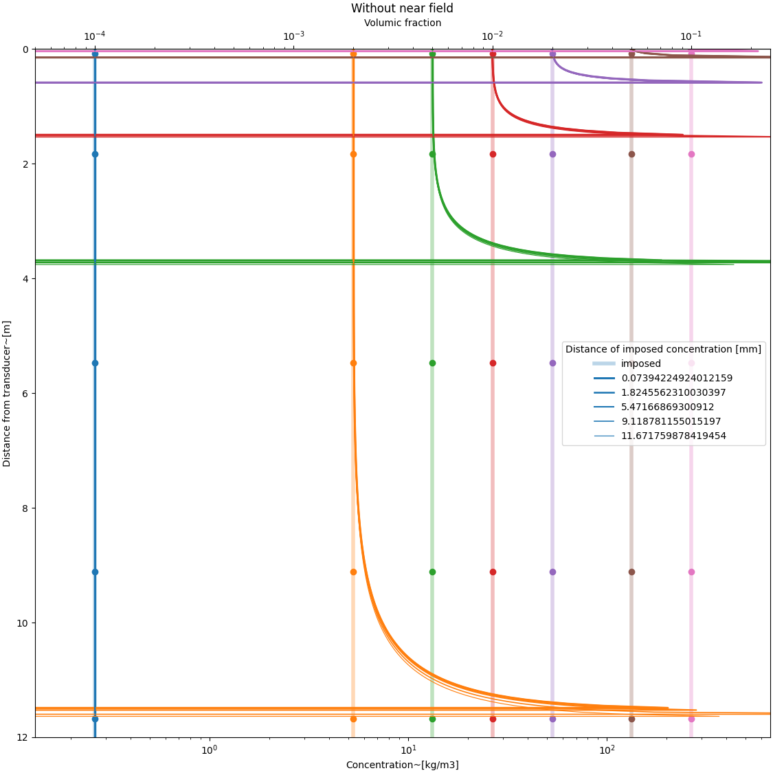
Influence of the imposed point in the integration

without near field function

psi = DM.near_field_theoretical(r, rn) * 0 + 1  # near field function
# defining a constant grain concentration profile
C = Phi[:, None] * rho * (r[None, :] * 0 + 1)
MSV = DM.create_MSvoltage(C, r, Xi, a_w, Ks, Kt, psi)
#
indexes = [2, 50, 150, 250, 320]

color = []
fig, ax = plt.subplots(
    1, 1, figsize=(fig_width_small, fig_width_small), constrained_layout=True
)
for i, phi in enumerate(Phi):
    if i == 0:
        a = plt.plot(C[i, :], r, lw=4, alpha=0.3, label="imposed")
    else:
        a = plt.plot(C[i, :], r, lw=4, alpha=0.3)
    color.append(a[0].get_color())
for j, index in enumerate(indexes):
    C0 = C[:, index]
    r0 = r[index]
    C_inferred, *_ = explicit_inversion(MSV, r, Xi, a_w, psi, C0, r0)
    for i, phi in enumerate(Phi):
        if i == 0:
            plt.plot(
                C_inferred[i, :], r, lw=2.5 - (j + 1) / 3, label=str(r0), color=color[i]
            )
        else:
            plt.plot(C_inferred[i, :], r, lw=2.5 - (j + 1) / 3, color=color[i])
        ax.scatter(C0[i], r0, color=color[i]),
plt.xlabel("Concentration~[kg/m3]")
plt.ylabel("Distance from transducer~[m]")
ax.set_xscale("log")
plt.xlim([0.5 * C.min(), 2.5 * C.max()])
plt.ylim([0, r.max()])
ax.invert_yaxis()
secax = ax.secondary_xaxis("top", functions=(C_to_phi, phi_to_C))
secax.set_xlabel("Volumic fraction")
plt.legend(title="Distance of imposed concentration [mm]")
plt.title("Without near field")

plt.show()

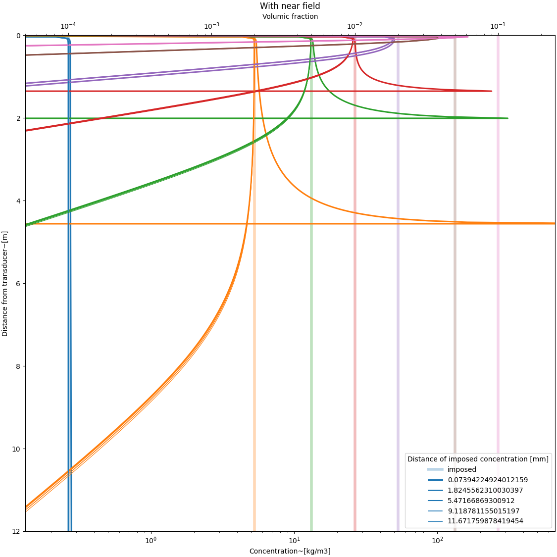
with near field function

psi = DM.near_field_theoretical(r, rn)  # near field function
# defining a constant grain concentration profile
C = Phi[:, None] * rho * (r[None, :] * 0 + 1)
MSV = DM.create_MSvoltage(C, r[None, :], Xi, a_w, Ks, Kt, psi[None, :])
#
color = []
fig, ax = plt.subplots(
    1, 1, figsize=(fig_width_small, fig_width_small), constrained_layout=True
)
for i, phi in enumerate(Phi):
    if i == 0:
        a = plt.plot(C[i, :], r, lw=4, alpha=0.3, label="imposed")
    else:
        a = plt.plot(C[i, :], r, lw=4, alpha=0.3)
    color.append(a[0].get_color())
for j, index in enumerate(indexes):
    C0 = C[:, index]
    r0 = r[index]
    C_inferred, *_ = explicit_inversion(MSV, r, Xi, a_w, psi * 0 + 1, C0, r0)
    for i, phi in enumerate(Phi):
        if i == 0:
            plt.plot(
                C_inferred[i, :], r, lw=2.5 - (j + 1) / 3, label=str(r0), color=color[i]
            )
        else:
            plt.plot(C_inferred[i, :], r, lw=2.5 - (j + 1) / 3, color=color[i])
plt.xlabel("Concentration~[kg/m3]")
plt.ylabel("Distance from transducer~[m]")
ax.set_xscale("log")
plt.xlim([0.5 * C.min(), 2.5 * C.max()])
plt.ylim([0, r.max()])
ax.invert_yaxis()
secax = ax.secondary_xaxis("top", functions=(C_to_phi, phi_to_C))
secax.set_xlabel("Volumic fraction")
plt.legend(title="Distance of imposed concentration [mm]")
plt.title("With near field")

plt.show()

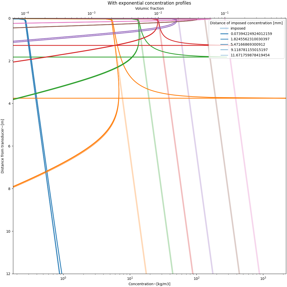
with real type concentration profiles

psi = DM.near_field_theoretical(r, rn)  # near field function
# C = (
#     Phi[:, None] * rho * np.exp(-r[None, :] / 1)
# )  # defining an exponentially decreasing profile
C = (
    Phi[:, None] * rho * np.exp(r[None, :] / 10)
)  # defining an exponentially increasing profile
# C = Phi[:, None] * rho * (r[None, :] * 0 + 1)  # defining sedimentation-like profile
# C[..., :230] = 0
#
MSV = DM.create_MSvoltage(C, r[None, :], Xi, a_w, Ks, Kt, psi[None, :])
#
color = []
fig, ax = plt.subplots(
    1, 1, figsize=(fig_width_small, fig_width_small), constrained_layout=True
)
for i, phi in enumerate(Phi):
    if i == 0:
        a = plt.plot(C[i, :], r, lw=4, alpha=0.3, label="imposed")
    else:
        a = plt.plot(C[i, :], r, lw=4, alpha=0.3)
    color.append(a[0].get_color())
for j, index in enumerate(indexes):
    C0 = C[:, index]
    r0 = r[index]
    C_inferred, *_ = explicit_inversion(MSV, r, Xi, a_w, psi * 0 + 1, C0, r0)
    for i, phi in enumerate(Phi):
        if i == 0:
            plt.plot(
                C_inferred[i, :], r, lw=2.5 - (j + 1) / 3, label=str(r0), color=color[i]
            )
        else:
            plt.plot(C_inferred[i, :], r, lw=2.5 - (j + 1) / 3, color=color[i])
        #
plt.xlabel("Concentration~[kg/m3]")
plt.ylabel("Distance from transducer~[m]")
ax.set_xscale("log")
plt.xlim([0.2 * C[:, -1].min(), 2.5 * C.max()])
plt.ylim([0, r.max()])
ax.invert_yaxis()
secax = ax.secondary_xaxis("top", functions=(C_to_phi, phi_to_C))
secax.set_xlabel("Volumic fraction")
plt.legend(title="Distance of imposed concentration [mm]")
plt.title("With exponential concentration profiles")

plt.show()