Note
Go to the end to download the full example code
Properties of a turbulent flow on a sinusoidal bottom#
In this tutorial, we show exemples using the
solve_turbulent_flow solver.
In particular, we focus on the calculation of the basal shear stress induced by a turbulent flow on a sinusoidal bottom, which is usefull for the sediment bed morphodynamics, in various flow configurations:
‘1D_unbounded’: 1D, unbounded turbulent flow (in practice capped by a rigid lid, that should be put far from the bed) [1, 2]
‘1D_freesurface’: 1D, turbulent flow capped by a free surface (typically river configuration) [1, 2]
‘1D_freeatmosphere’: 1D, turbulent flow capped by a stratified flow (typically atmopshere configuration) [3]
‘2D_unbounded’: 2D, unbounded turbulent flow (in practice capped by a rigid lid, that should be put far from the bed) [1, 2, 3]
For details on the flow theoretical modelling, please refer to the references below:
One-dimensional case – unbounded regime#
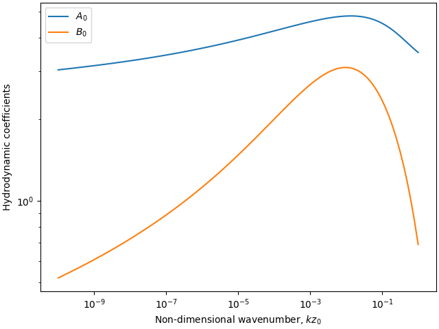
Basal shear stress coefficients#
model = '1D_unbounded'

eta_H = 10
eta_0_vals = np.logspace(-10, 0, 100)
eta = 0
#
coeffs = np.zeros((2, eta_0_vals.size))
for i, eta_0 in enumerate(eta_0_vals):
    parameters = {'eta_H': eta_H, 'eta_0': eta_0}
    solution_function = solve_turbulent_flow(model, parameters)
    # solution at the bottom surface
    solution = solution_function(eta)
    A0, B0 = np.real(solution[2]), np.imag(solution[2])
    coeffs[:, i] = [A0, B0]

fig, ax = plt.subplots(1, 1, constrained_layout=True)
ax.plot(eta_0_vals, coeffs[0, :], label='$A_{0}$')
ax.plot(eta_0_vals, coeffs[1, :], label='$B_{0}$')
#
ax.set_xscale('log')
ax.set_yscale('log')
ax.set_xlabel(r'Non-dimensional wavenumber, $k z_{0}$')
ax.set_ylabel('Hydrodynamic coefficients')
plt.legend()
plt.show()
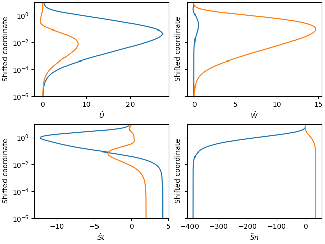
Vertical profiles#
eta = np.logspace(np.log10(1e-6), np.log10(0.95*eta_H), 1000)
eta_0 = 1e-4
parameters = {'eta_H': eta_H, 'eta_0': eta_0}

solution_function = solve_turbulent_flow(
    model, parameters, atol=1e-14, rtol=1e-14)
solution = solution_function(eta)

labels = [r'$\~U$', r'$\~W$', r'$\~St$', r'$\~Sn$']
fig, axarr = plt.subplots(2, 2, constrained_layout=True, sharey=True)
for i, (ax, sol, label) in enumerate(zip(axarr.flatten(), solution, labels)):
    if i == 0:
        ax.semilogy(np.real(sol + mu_prime(eta, eta_0, Kappa=0.4)), eta)
        ax.semilogy(np.imag(sol + mu_prime(eta, eta_0, Kappa=0.4)), eta)
    else:
        ax.semilogy(np.real(sol), eta)
        ax.semilogy(np.imag(sol), eta)
    ax.set_ylim(1e-6, 10)
    ax.set_ylabel('Shifted coordinate')
    ax.set_xlabel(label)
plt.show()
/opt/hostedtoolcache/Python/3.11.6/x64/lib/python3.11/site-packages/scipy/integrate/_ivp/common.py:47: UserWarning: At least one element of `rtol` is too small. Setting `rtol = np.maximum(rtol, 2.220446049250313e-14)`.
  warn("At least one element of `rtol` is too small. "
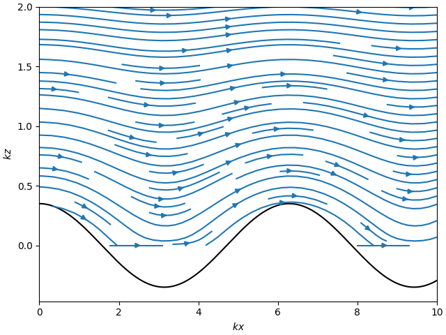
streamlines#
# topography parameters
k_xi = 0.35
k_x = np.linspace(0, 10, 500)
kZ = k_xi*np.real(np.exp(1j*k_x))

# calculating solution on linearly distributed vertical coordinates
eta = np.linspace(1e-10, 2, 1000)
solution = solution_function(eta)

# calculating velocity field from the solution
Ux = np.real(mu(eta[:, None], eta_0)
             + k_xi*np.exp(1j*k_x[None, :]) * solution[0, :][:, None])
Uz = np.real(k_xi*np.exp(1j*k_x[None, :]) * solution[1, :][:, None])
U = np.sqrt(Ux**2 + Uz**2)

mask = (eta[:, None] <= kZ[None, :])
Ux = np.ma.array(Ux, mask=mask)
Uz = np.ma.array(Uz, mask=mask)

# figure
fig, ax = plt.subplots(1, 1, constrained_layout=True)
plt.plot(k_x, kZ, color='k')
ax.streamplot(k_x, eta, Ux, Uz)
ax.set_xlabel('$k x$')
ax.set_ylabel('$k z$')
plt.show()
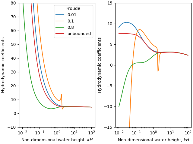
One-dimensional case – interaction with the free surface#
Dependency of the basal shear stress coefficients on the water height#
eta_H_vals = np.logspace(-2, 2, 100)
Froudes = np.array([0.01, 0.1, 0.8, None])
H_z0_ratio = 1e3
eta = 0
#
coeffs = np.zeros((2, eta_H_vals.size, Froudes.size))
for i, eta_H in enumerate(eta_H_vals):
    eta_0 = eta_H/H_z0_ratio
    for j, Fr in enumerate(Froudes):
        if Fr is None:
            model = '1D_unbounded'
            parameters = {'eta_H': eta_H, 'eta_0': eta_0}
        else:
            model = '1D_freesurface'
            parameters = {'eta_H': eta_H, 'eta_0': eta_0, 'Fr': Fr}
        solution_function = solve_turbulent_flow(model, parameters)
        solution = solution_function(eta)
        #
        A0, B0 = np.real(solution[2]), np.imag(solution[2])
        coeffs[:, i, j] = [A0, B0]

# Figure
fig, axarr = plt.subplots(1, 2, constrained_layout=True, sharex=True)
for j, Fr in enumerate(Froudes):
    axarr[0].plot(eta_H_vals, coeffs[0, :, j], label=str(Fr)
                  if Fr is not None else 'unbounded')
    axarr[1].plot(eta_H_vals, coeffs[1, :, j])
#
for ax in axarr:
    ax.set_xscale('log')
    ax.set_xlabel(r'Non-dimensional water height, $k H$')
    ax.set_ylabel('Hydrodynamic coefficients')
axarr[0].set_ylim(-10, 80)
axarr[1].set_ylim(-15, 15)
axarr[0].legend(title='Froude')
plt.show()
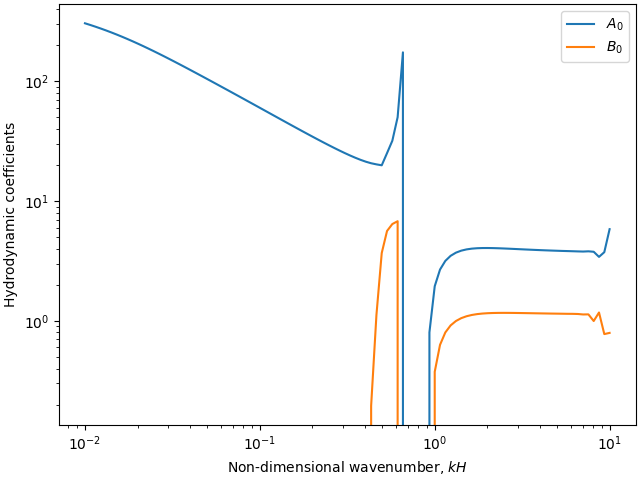
One-dimensional case – interaction with the free surface topped by a stratified free atmosphere#
Dependency of the basal shear stress coefficients on the bottom perturbation orientation#
model = '1D_freeatmosphere'

eta_0 = 1e-6
eta_H_vals = np.logspace(-2, 1, 100)
eta_B_vals = 2*eta_H_vals
Fr = np.sqrt(0.7)
eta = 0

coeffs = np.zeros((2, eta_H_vals.size))
for i, (eta_H, eta_B) in enumerate(zip(eta_H_vals, eta_B_vals)):
    # #### turbulent flow
    parameters = {'eta_H': eta_H, 'eta_0': eta_0, 'Fr': Fr, 'eta_B': eta_B}
    solution_function, _ = solve_turbulent_flow(model, parameters)
    solution = solution_function(eta)
    #
    A0, B0 = np.real(solution[2]), np.imag(solution[2])
    coeffs[:, i] = [A0, B0]


fig, ax = plt.subplots(1, 1, constrained_layout=True, sharex=True)
ax.plot(eta_H_vals, coeffs[0, :], label='$A_{0}$')
ax.plot(eta_H_vals, coeffs[1, :], label='$B_{0}$')
ax.set_xscale('log')
ax.set_yscale('log')
ax.set_xlabel(r'Non-dimensional wavenumber, $k H$')
ax.set_ylabel('Hydrodynamic coefficients')
plt.legend()
plt.show()
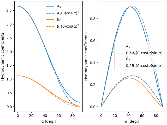
Two-dimensional case – unbounded regime#
Dependency of the basal shear stress coefficients on the bottom perturbation orientation#
model = '2D_unbounded'

eta_H = 10
eta_0 = 1e-6
alpha_vals = np.linspace(0, 90, 30)
eta = 0

coeffs = np.zeros((4, alpha_vals.size))
for i, alpha in enumerate(alpha_vals):
    parameters = {'eta_H': eta_H, 'eta_0': eta_0, 'alpha': alpha}
    solution_function = solve_turbulent_flow(
        model, parameters, rtol=1e-15, atol=1e-15)
    solution = solution_function(eta)
    #
    Ax_m, Bx_m = np.real(solution[3]), np.imag(solution[3])
    Ay_m, By_m = np.real(solution[4]), np.imag(solution[4])
    coeffs[:, i] = [Ax_m, Bx_m, Ay_m, By_m]


fig, axarr = plt.subplots(1, 2, constrained_layout=True, sharex=True)
a,  = axarr[0].plot(alpha_vals, coeffs[0, :], label='$A_{x}$')
axarr[0].plot(alpha_vals, Ax_geo(alpha_vals, coeffs[0, 0]),
              color=a.get_color(), ls='--', label=r'$A_{x}(0)\cos(\alpha)^{2}$')
b, = axarr[0].plot(alpha_vals, coeffs[1, :], label='$B_{x}$')
axarr[0].plot(alpha_vals, Bx_geo(alpha_vals, coeffs[1, 0]),
              color=b.get_color(), ls='--', label=r'$B_{x}(0)\cos(\alpha)^{2}$')
#
a, = axarr[1].plot(alpha_vals, coeffs[2, :], label='$A_{y}$')
axarr[1].plot(alpha_vals, Ay_geo(alpha_vals, coeffs[0, 0]),
              color=a.get_color(), ls='--',  label=r'0.5$A_{x}(0)\cos(\alpha)\sin(\alpha)$')
b, = axarr[1].plot(alpha_vals, coeffs[3, :], label='$B_{y}$')
axarr[1].plot(alpha_vals, By_geo(alpha_vals, coeffs[1, 0]),
              color=a.get_color(), ls='--', label=r'0.5$B_{x}(0)\cos(\alpha)\sin(\alpha)$')

axarr[0].set_ylabel('Hydrodynamic coefficients')
axarr[0].set_xlabel(r'$\alpha$ [deg.]')
axarr[0].legend()
axarr[1].set_ylabel('Hydrodynamic coefficients')
axarr[1].set_xlabel(r'$\alpha$ [deg.]')
axarr[1].legend()

plt.show()
Total running time of the script: (2 minutes 53.691 seconds)