From wind data to sand fluxes and dune orientations

In this tutorial, we show on the use pydune functions to go from wind data, to the calculation of sand fluxes, and then to dune properties.

import numpy as np
import matplotlib.pyplot as plt
from pydune.data_processing import load_netcdf
from pydune.data_processing import velocity_to_shear, plot_flux_rose, plot_wind_rose
from pydune.math import (
    cartesian_to_polar,
    tand,
    make_angular_PDF,
    make_angular_average,
    vector_average,
)

Loading and plotting the wind data

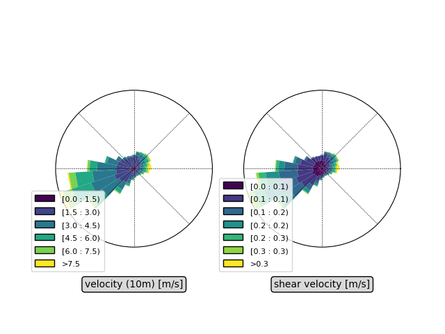
We first load the data, and caculate the shear velocity using the law of the wall:

data = load_netcdf(["../src/ERA5Land2020to2021_Taklamacan.netcdf"])
z_ERA = 10  # height of wind data in the dataset, [m]
#
velocity, orientation = cartesian_to_polar(data["u10"][:, 0, 0], data["v10"][:, 0, 0])
shear_velocity = velocity_to_shear(velocity, z_ERA)

# figure
bins_shear = [0, 0.1, 0.15, 0.2, 0.25, 0.3, 0.35]
bins = [0, 1.5, 3, 4.5, 6, 7.5]
bbox_label = dict(boxstyle="round", facecolor=(0, 0, 0, 0.15), edgecolor=(0, 0, 0, 1))

fig, axarr = plt.subplots(1, 2, constrained_layout=True)
a = plot_wind_rose(
    orientation,
    velocity,
    bins,
    axarr[0],
    fig,
    opening=1,
    nsector=25,
    cmap=plt.cm.viridis,
    legend=True,
    label="velocity (10m) [m/s]",
    props=bbox_label,
)
a.set_legend(bbox_to_anchor=(-0.15, -0.15))
a = plot_wind_rose(
    orientation,
    shear_velocity,
    bins_shear,
    axarr[1],
    fig,
    opening=1,
    nsector=25,
    cmap=plt.cm.viridis,
    legend=True,
    label="shear velocity [m/s]",
    props=bbox_label,
)
a.set_legend(bbox_to_anchor=(-0.15, -0.15))
plt.show()

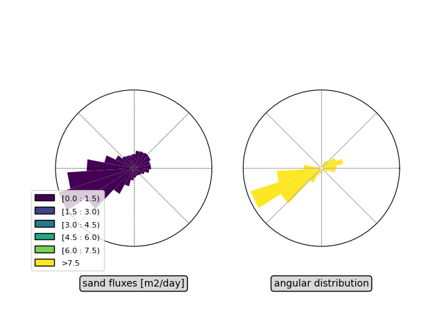
Calculating the sand fluxes

We then calculate sand fluxes using the quartic law:

from pydune.physics import quartic_transport_law

# # Parameters
sectoday = 24 * 3600
rho_g = 2.65e3  # grain density
rho_f = 1  # fluid density
g = 9.81  # [m/s2]
grain_diameters = 180e-6  # grain size [m]
bed_porosity = 0.6  # bed porosity
#
Q = (
    np.sqrt((rho_g - rho_f) * g * grain_diameters / rho_f) * grain_diameters
)  # characteristic flux [m2/s]
shield_th_quartic = 0.0035  # threshold shield numbers for the quartic

# shield number
shield = (rho_f / ((rho_g - rho_f) * g * grain_diameters)) * shear_velocity**2
# dimensional sand flux, [m2/day]
sand_flux = (
    (1 / bed_porosity) * Q * quartic_transport_law(shield, shield_th_quartic) * sectoday
)
# angular distribution
angular_PDF, angles = make_angular_PDF(orientation, sand_flux)

DP = np.mean(sand_flux)  # Drift potential, [m2/day]
# Resultant drift direction [deg.] / Resultant drift potential, [m2/day]
RDD, RDP = vector_average(orientation, sand_flux)

print(
    r"""
     - DP =  {: .1f} [m2/day]
     - RDP = {: .1f} [m2/day]
     - RDP/DP = {: .2f}
     - RDD = {: .0f} [deg.]

""".format(
        DP, RDP, RDP / DP, RDD % 360
    )
)

# figure
bins_flux = [0, 0.3, 0.6, 0.9, 1.2, 1.5]
fig, axarr = plt.subplots(1, 2, constrained_layout=True)
a = plot_wind_rose(
    orientation,
    sand_flux,
    bins,
    axarr[0],
    fig,
    opening=1,
    nsector=25,
    cmap=plt.cm.viridis,
    legend=True,
    label="sand fluxes [m2/day]",
    props=bbox_label,
)
a.set_legend(bbox_to_anchor=(-0.15, -0.15))
a = plot_flux_rose(
    angles,
    angular_PDF,
    axarr[1],
    fig,
    opening=1,
    label="angular distribution",
    nsector=25,
    props=bbox_label,
)
plt.show()

- DP =   0.1 [m2/day]
- RDP =  0.0 [m2/day]
- RDP/DP =  0.32
- RDD =  219 [deg.]

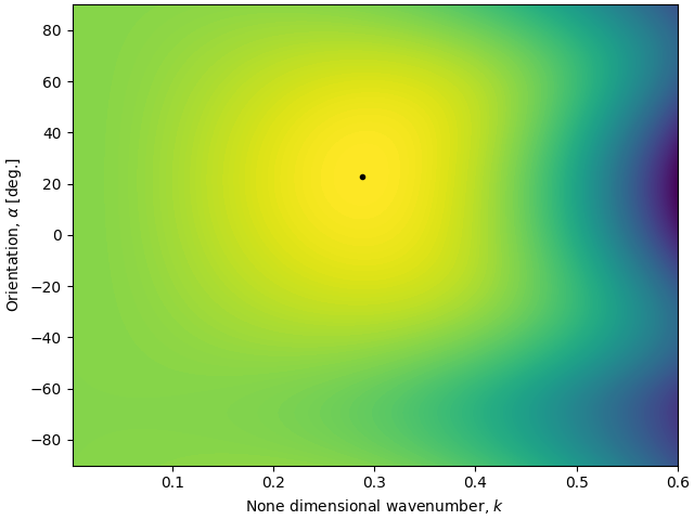
Properties of incipient dunes

We compute the propoerties of incipient dunes (in the linear regime) using the model of Gadal et al. 2019.

[1] Gadal, C., Narteau, C., Du Pont, S. C., Rozier, O., & Claudin, P. (2019). Incipient bedforms in a bidirectional wind regime. Journal of Fluid Mechanics, 862, 490-516.

from pydune.physics import bedinstability_2D as BI2D
from pydune.physics import Ax_geo, Bx_geo, Ay_geo, By_geo, A0_approx, B0_approx

# parameters
k = np.linspace(0.001, 0.6, 300)  # range of explored wavelengths, non-dimensional
alpha = np.linspace(-90, 90, 181)  # range of explored orientations, non-dimensional
mu = tand(35)  # friction coefficient
delta = 0  # diffusion coefficient
z0 = 1e-3  # hydrodynamic roughness


def Ax(k, alpha):
    return Ax_geo(alpha, A0_approx(k * z0))


def Bx(k, alpha):
    return Bx_geo(alpha, B0_approx(k * z0))


def Ay(k, alpha):
    return Ay_geo(alpha, A0_approx(k * z0))


def By(k, alpha):
    return By_geo(alpha, A0_approx(k * z0))


# threshold shear velocity [m/s]
shear_velocity_th = np.sqrt(
    shield_th_quartic / (rho_f / ((rho_g - rho_f) * g * grain_diameters))
)
# average velocity ratio by angle bin
r, _ = make_angular_average(
    orientation,
    np.where(shear_velocity > shear_velocity_th, shear_velocity / shear_velocity_th, 1),
)
# characteristic average velocity ratio by angle bin (just when its always the threshold)
r_car, _ = make_angular_average(
    orientation[shear_velocity > shear_velocity_th],
    shear_velocity[shear_velocity > shear_velocity_th] / shear_velocity_th,
)

# dimensional constants
Lsat = 2.2 * ((rho_g - rho_f) / rho_f) * grain_diameters  # saturation length [m]
Q_car = (
    DP * angular_PDF / (1 - 1 / r**2)
)  # Characteristic flux of the instability (without threshold), [m2/day]
Q_car[np.isnan(Q_car)] = 0

# Calculation of the growth rate
sigma = BI2D.temporal_growth_rate_multi(
    k[None, :, None],
    alpha[:, None, None],
    Ax,
    Ay,
    Bx,
    By,
    r_car,
    mu,
    delta,
    angles[None, None, :],
    Q_car[None, None, :],
    axis=-1,
)


# Properties of the most unstable mode (dimensional)
i_amax, i_kmax = np.unravel_index(sigma.argmax(), sigma.shape)
sigma_max = sigma.max() / Lsat**2
alpha_max = alpha[i_amax]
k_max = k[i_kmax] / Lsat
c_max = Lsat * BI2D.temporal_celerity_multi(
    Lsat * k_max, alpha_max, Ax, Ay, Bx, By, r_car, mu, delta, angles, Q_car, axis=-1
)

fig, ax = plt.subplots(1, 1, constrained_layout=True)
ax.contourf(k, alpha, sigma / Lsat**2, levels=200)
ax.plot(k[i_kmax], alpha[i_amax], "k.")
ax.set_xlabel("None dimensional wavenumber, $k$")
ax.set_ylabel(r"Orientation, $\alpha$ [deg.]")
plt.show()

print(
    r""" The properties of the most unstable mode are:
     - orientation: {:.0f} [deg.]
     - wavenumber :{:.1e}  [/m]
     - wavelength : {:.1e} [m]
     - growth rate :  {:.1e} [/day]
     - migration velocity: {:.1e} [m/day]

""".format(
        alpha_max + 90, k_max, 2 * np.pi / k_max, sigma_max, c_max
    )
)

/home/runner/work/pydune/pydune/examples/tutorials/plot_windtofluxtodune.py:198: RuntimeWarning: invalid value encountered in divide
  DP * angular_PDF / (1 - 1 / r**2)
 The properties of the most unstable mode are:
     - orientation: 113 [deg.]
     - wavenumber :2.7e-01  [/m]
     - wavelength : 2.3e+01 [m]
     - growth rate :  5.2e-03 [/day]
     - migration velocity: -8.3e-02 [m/day]

Properties of mature dunes

We then compute the two possible mature dune orientations using the model of Courrech du Pont et al. 2014.

[1] Courrech du Pont, S., Narteau, C., & Gao, X. (2014). Two modes for dune orientation. Geology, 42(9), 743-746.

from pydune.physics.dune.courrechdupont2014 import (
    elongation_direction,
    MGBNT_orientation,
)


Alpha_E = elongation_direction(angles, angular_PDF)
Alpha_BI = MGBNT_orientation(angles, angular_PDF)

print(
    r""" The properties of the mature dunes are:
     - Elongation direction: {: .0f} [deg]
     - MGBNT crest orientation: {: .0f} [deg]

""".format(
        Alpha_E, Alpha_BI
    )
)

The properties of the mature dunes are:
    - Elongation direction:  224 [deg]
    - MGBNT crest orientation:  109 [deg]